概念

LayerNorm

LayerNorm是一种神经网络中的归一化技术，用于稳定和加速训练过程。它不像BatchNorm那样在整个批次的样本间归一化，而是在单个样本的不同特征维度间进行归一化。

GELU

GELU是一种激活函数，它结合了ReLU的正部分和基于输入概率的随机门控思想。不同于ReLU的硬性"截断"（小于0输出0），GELU通过输入值的概率来"软化"门控效果。

def gelu(x):
  """Gaussian Error Linear Unit.

  This is a smoother version of the RELU.
  Original paper: https://arxiv.org/abs/1606.08415
  Args:
    x: float Tensor to perform activation.

  Returns:
    `x` with the GELU activation applied.
  """
  cdf = 0.5 * (1.0 + tf.tanh(
      (np.sqrt(2 / np.pi) * (x + 0.044715 * tf.pow(x, 3)))))
  return x * cdf

PE

位置编码是为序列数据（如文本）中的每个位置添加一个表示其顺序信息的向量。由于Transformer的自注意力机制本身没有顺序概念（是排列不变的），需要通过位置编码来注入序列的顺序信息。

# 最简正弦位置编码实现
def sinusoidal_encoding(seq_len, d_model):
    """直接计算正弦位置编码"""
    pe = torch.zeros(seq_len, d_model)
    position = torch.arange(0, seq_len).float().unsqueeze(1)
    
    # 计算频率项
    div_term = torch.exp(
        torch.arange(0, d_model, 2).float() * 
        -(math.log(10000.0) / d_model)
    )
    
    pe[:, 0::2] = torch.sin(position * div_term)
    pe[:, 1::2] = torch.cos(position * div_term)
    return pe  # [seq_len, d_model]

Multi-Head Attention

Multi-Head Attention = 多个低维注意力头并行 = 每个头关注不同的子空间模式 = 最后 concat 再线性融合

class MultiHeadAttention(nn.Module):
    def __init__(self, embed_dim, num_heads):
        super().__init__()
        assert embed_dim % num_heads == 0, "embed_dim 必须能被 num_heads 整除"

        self.embed_dim = embed_dim
        self.num_heads = num_heads
        self.head_dim = embed_dim // num_heads

        # 为了简单，给 Q、K、V 各自一个线性层
        self.q_proj = nn.Linear(embed_dim, embed_dim)
        self.k_proj = nn.Linear(embed_dim, embed_dim)
        self.v_proj = nn.Linear(embed_dim, embed_dim)

        # 多头输出拼接后，再过一个输出线性层
        self.out_proj = nn.Linear(embed_dim, embed_dim)

    def forward(self, q, k, v):
        """
        q, k, v: 形状都是 (batch_size, seq_len, embed_dim)
        返回:    (batch_size, seq_len, embed_dim)
        """
        batch_size, seq_len, _ = q.size()

        # 1. 线性映射到 Q, K, V
        Q = self.q_proj(q)  # (B, L, E)
        K = self.k_proj(k)  # (B, L, E)
        V = self.v_proj(v)  # (B, L, E)

        # 2. reshape + transpose，拆成多头
        # 先变成 (B, L, H, D)，再转成 (B, H, L, D)
        def split_heads(x):
            return x.view(batch_size, seq_len, self.num_heads, self.head_dim).transpose(1, 2)

        Q = split_heads(Q)  # (B, H, L, D)
        K = split_heads(K)  # (B, H, L, D)
        V = split_heads(V)  # (B, H, L, D)

        # 3. 计算缩放点积注意力
        # scores: (B, H, L, L)
        scores = torch.matmul(Q, K.transpose(-2, -1)) / math.sqrt(self.head_dim)
        attn = torch.softmax(scores, dim=-1)  # 对最后一个维度做 softmax

        # 4. 用注意力权重加权 V
        # context: (B, H, L, D)
        context = torch.matmul(attn, V)

        # 5. 把多头拼回去
        # 先变回 (B, L, H, D)，再合并 H、D -> E
        context = context.transpose(1, 2).contiguous().view(batch_size, seq_len, self.embed_dim)

        # 6. 最后再过一个线性层
        out = self.out_proj(context)  # (B, L, E)
        return out

mha = MultiHeadAttention(embed_dim=8, num_heads=2)
# 随机造一串序列特征
x = torch.randn(2, 4, 8)
# 自注意力：q = k = v = x
out = mha(x, x, x)
print("输入形状:", x.shape)   # (2, 4, 8)
print("输出形状:", out.shape)  # (2, 4, 8)

GQA与MQA、MLA

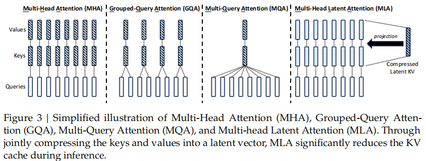
https://sebastianraschka.com/llms-from-scratch/ch04/05_mla/

这是一种高效的自注意力机制变体，特别适合于需要处理长序列的场景。传统自注意力（Transformer）的计算复杂度是 O(n²)，MLA通过引入潜在表示（Latent Representation） 来降低计算量。关键区别在于：

• 传统Attention: Q, K, V 都直接从输入x线性变换得到
• MLA: 只有Q直接从x得到，K和V先投影到一个低维潜在空间，再投影回来，W_DKV 将输入压缩到低维空间 (latent_dim 通常比 d_out 小很多)，主要的矩阵乘法在低维空间进行存储和缓存

class MultiHeadLatentAttention(nn.Module):
    def __init__(self, d_in, d_out, dropout, num_heads,
                 qkv_bias=False, latent_dim=None):
        super().__init__()
        assert d_out % num_heads == 0, "d_out must be divisible by num_heads"

        self.d_out = d_out
        self.num_heads = num_heads
        self.head_dim = d_out // num_heads
        self.latent_dim = latent_dim if latent_dim is not None else max(16, d_out // 8)

        # Projections
        self.W_query = nn.Linear(d_in, d_out, bias=qkv_bias)              # per-head Q
        self.W_DKV = nn.Linear(d_in, self.latent_dim, bias=qkv_bias)    # down to latent C
        self.W_UK = nn.Linear(self.latent_dim, d_out, bias=qkv_bias)   # latent -> per-head K
        self.W_UV = nn.Linear(self.latent_dim, d_out, bias=qkv_bias)   # latent -> per-head V

        self.out_proj = nn.Linear(d_out, d_out)
        self.dropout = nn.Dropout(dropout)

        ####################################################
        # Latent-KV cache
        self.register_buffer("cache_c_kv", None, persistent=False)
        self.ptr_current_pos = 0
        ####################################################

    def reset_cache(self):
        self.cache_c_kv = None
        self.ptr_current_pos = 0

    @staticmethod
    def _reshape_to_heads(x, num_heads, head_dim):
        # (b, T, d_out) -> (b, num_heads, T, head_dim)
        bsz, num_tokens, _ = x.shape
        return x.view(bsz, num_tokens, num_heads, head_dim).transpose(1, 2).contiguous()

    def forward(self, x, use_cache=False):
        b, num_tokens, _ = x.shape
        num_heads = self.num_heads
        head_dim = self.head_dim

        # 1) Project to queries (per-token, per-head) and new latent chunk
        queries_all = self.W_query(x)  # (b, T, d_out)
        latent_new = self.W_DKV(x)  # (b, T, latent_dim)

        # 2) Update latent cache and choose latent sequence to up-project
        if use_cache:
            if self.cache_c_kv is None:
                latent_total = latent_new
            else:
                latent_total = torch.cat([self.cache_c_kv, latent_new], dim=1)
            self.cache_c_kv = latent_total
        else:
            latent_total = latent_new

        # 3) Up-project latent to per-head keys/values (then split into heads)
        keys_all = self.W_UK(latent_total)   # (b, T_k_total, d_out)
        values_all = self.W_UV(latent_total)   # (b, T_k_total, d_out)

        # 4) Reshape to heads
        queries = self._reshape_to_heads(queries_all, num_heads, head_dim)
        keys = self._reshape_to_heads(keys_all, num_heads, head_dim)
        values = self._reshape_to_heads(values_all, num_heads, head_dim)

        # 5) Scaled dot-product attention with causal mask
        attn_scores = torch.matmul(queries, keys.transpose(-2, -1))

        num_tokens_Q = queries.shape[-2]
        num_tokens_K = keys.shape[-2]
        device = queries.device
        if use_cache:
            q_positions = torch.arange(
                self.ptr_current_pos,
                self.ptr_current_pos + num_tokens_Q,
                device=device,
                dtype=torch.long,
            )
            self.ptr_current_pos += num_tokens_Q
        else:
            q_positions = torch.arange(num_tokens_Q, device=device, dtype=torch.long)
            self.ptr_current_pos = 0
        k_positions = torch.arange(num_tokens_K, device=device, dtype=torch.long)
        mask_bool = q_positions.unsqueeze(-1) < k_positions.unsqueeze(0)

        # Use the mask to fill attention scores
        attn_scores.masked_fill_(mask_bool, -torch.inf)

        attn_weights = torch.softmax(attn_scores / keys.shape[-1]**0.5, dim=-1)
        attn_weights = self.dropout(attn_weights)

        # Shape: (b, num_tokens, num_heads, head_dim)
        context_vec = (attn_weights @ values).transpose(1, 2)

        # Combine heads, where self.d_out = self.num_heads * self.head_dim
        context_vec = context_vec.contiguous().view(b, num_tokens, self.d_out)
        context_vec = self.out_proj(context_vec)  # optional projection

        return context_vec

RoPE

RoPE的核心思想是：通过复数旋转的方式将位置信息注入到注意力计算中。与传统的位置嵌入（直接加到token embedding上）不同，RoPE通过旋转向量的方式来编码位置信息。

把每个向量的最后一维拆成很多个二维平面（每 2 维一组）。在每个二维平面里，对位置 i 的向量应用一个与 i 相关的旋转角度$\theta_i$

def apply_rope(x, freqs):
    """
    x: [batch, seq_len, num_heads, head_dim]
    freqs: [1, seq_len, 1, head_dim//2] 旋转频率
    """
    # 将x分成实部和虚部（或理解为cos和sin部分）
    x_complex = torch.view_as_complex(
        x.float().reshape(*x.shape[:-1], -1, 2)
    )
    
    # 应用旋转
    freqs_cis = torch.polar(torch.ones_like(freqs), freqs)
    x_out = torch.view_as_real(x_complex * freqs_cis)
    
    return x_out.reshape(*x.shape)

RMSNorm

移除均值中心化,减少30-40%的计算量

class RMSNorm(torch.nn.Module):
    def __init__(self, dim: int, eps: float = 1e-6):
        super().__init__()
        self.eps = eps
        self.weight = nn.Parameter(torch.ones(dim))  # 可学习的γ参数

    def _norm(self, x):
        # x: [..., dim]
        # RMS(x) = sqrt(mean(x^2))
        return x * torch.rsqrt(x.pow(2).mean(-1, keepdim=True) + self.eps)

    def forward(self, x):
        output = self._norm(x.float()).type_as(x)
        return output * self.weight

MoE

在计算量差不多的情况下，让模型“变大、变聪明、又更会分工”。

MoE：有很多个专家子网络，但每个输入只激活其中少数几个（比如 top-1、top-2 专家）。

结果：总参数量很大（模型“容量”很强）；但一次前向只用少数专家，实际计算量接近少数专家之和，而不是所有专家之和。在相似算力下，获得比普通模型更高的表达能力。

同时让模型通过门控网络学习不同的专家模式

class SimpleMoE(nn.Module):
    def __init__(self, dim, num_experts, hidden_dim):
        """
        dim:         输入和输出的特征维度
        num_experts: 专家数量
        hidden_dim:  每个专家内部的隐层维度
        """
        super().__init__()
        self.dim = dim
        self.num_experts = num_experts
        self.hidden_dim = hidden_dim

        # 构造多个专家，每个专家都是一个小的前馈网络
        self.experts = nn.ModuleList([
            nn.Sequential(
                nn.Linear(dim, hidden_dim),
                nn.ReLU(),
                nn.Linear(hidden_dim, dim),
            )
            for _ in range(num_experts)
        ])

        # 门控网络：把输入映射到 num_experts 维度，作为专家权重的 logits
        self.gate = nn.Linear(dim, num_experts)

    def forward(self, x):
        """
        x: (batch_size, seq_len, dim)
        返回: (batch_size, seq_len, dim)
        """
        batch_size, seq_len, dim = x.shape
        assert dim == self.dim

        # 1. 门控网络计算每个位置对各个专家的权重
        #    gate_logits: (B, L, E)
        gate_logits = self.gate(x)
        gate_weights = F.softmax(gate_logits, dim=-1)  # (B, L, E)

        # 2. 所有专家分别对同一个 x 前向
        #    expert_outputs 是 list，每个元素 (B, L, D)
        expert_outputs = [expert(x) for expert in self.experts]

        # 3. 堆叠成一个张量，方便做加权求和
        #    stacked: (B, L, E, D)
        stacked = torch.stack(expert_outputs, dim=2)

        # 4. 按门控权重做加权求和
        #    gate_weights: (B, L, E) -> (B, L, E, 1)
        gate_expanded = gate_weights.unsqueeze(-1)

        #    加权求和 over E 维度
        out = torch.sum(gate_expanded * stacked, dim=2)  # (B, L, D)

        return out

强化学习概念

https://hrl.boyuai.com/chapter/2/ppo%E7%AE%97%E6%B3%95

PPO 是一种策略梯度强化学习算法，经常用在 RLHF 里。 它的核心思想是：用人类反馈训练一个 reward model，然后在旧策略附近做小步更新，提高奖励高的回答的概率、降低奖励低的回答。 为了防止一步走太远，PPO 通过 clip 或者 KL 惩罚约束新旧策略的差距，这样训练会比较稳定，不容易崩。

DPO 不再“先训奖励模型再做 RL”，而是直接用人类的成对偏好数据来训练策略，是一种“把偏好学习写成监督学习”的方法。

DPO 是最近比较流行的一种对齐方法，叫 Direct Preference Optimization。它假设我们有很多 (prompt, 好回答, 坏回答) 的偏好数据。在训练时，不训练单独的 reward model，而是直接用一个 logistic 风格的 loss，让模型在同一个 prompt 下，对“更好的回答”给更高的 log 概率，对“更差的回答”给更低的 log 概率。同时会加一个和 reference model 的 KL 正则，约束新模型不要离原始模型太远。这样整个对齐过程就变成“类似监督学习的分类/排序问题”，实现简单、稳定性也很好。

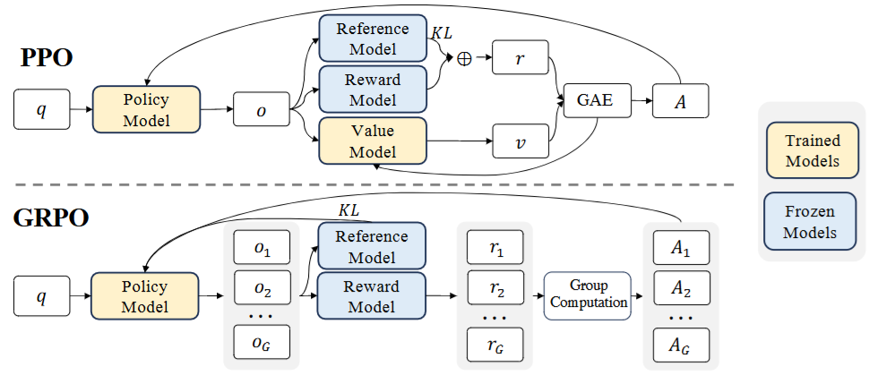
PPO 中的reward model通常是一个与策略模型大小相当的模型，这带来了显著的内存和计算负担。 GRPO 全称 Group Relative Policy Optimization，可以看成是对 PPO 思路的一个简化。对每个 prompt，我们让当前策略一次性生成多条候选回答，用奖励模型或者打分函数给它们打分。然后用“比组内平均分高多少”作为优势来更新策略：比平均好的回答概率提高，比平均差的回答概率降低。这样一来，不需要单独的 value function，优势估计简单，而且天然是相对的，更稳定、比较适合大规模分布式训练。